SIMD-pathtracer
Project Checkpoint: SIMD Parallelization of a Path Tracer
Authors: Michelle Ma, Rain Du
Abstract
We implemented a SIMD ray tracer in ISPC on CPU. In this report, we will analyze the challenges and optimizations of our algorithm, discuss how each optimization resolves issues such as locality and vector utilization problems. For our deliverables, we will present rendered images, performance comparison graphs, an interactive path tracer application and its source code, and our poster for easy comparison and visualization. Our implementation achieved a 175x speedup on a 4 core Macbook 2019 13”.
Background
Path tracing is a classic and well-developed method to render convincing images of 3D scenes based on their mathematical descriptions. Path tracing is widely used in industries like animation, due to the high fidelity images it can generate, but its high computational cost prevented it from being used in many other - mostly interactive - applications. Fortunately the algorithm itself does not impose much data dependency, allowing people to continue researching ways to accelerate path tracing through parallelization. Historically the most common way to parallelize a path tracer is to run it across multiple CPU processors, but utilizing SIMD parallelization is also an attractive direction.
Below is a summarization of the path tracing algorithm and an overview of our existing sequential implementation.
Algorithm Overview
In the initial sequential implementation, we have a function that traces all rays in a scene. It first generates all rays as a data structure ray task, and the helper trace_ray function is called on individual corresponding ray struct in order, with each function call tracing a ray starting from a pixel (there can be multiple rays starting from a pixel), reflecting and refracting through bouncing with the objects of different materials in the scene. Each time the ray touches an object, a new ray will be generated for the old ray (due to reflection or refraction), and trace_ray is called recursively with the newly bounced ray. Once the subsequent rays finally arrived at the source of the light, has too small of a contribution to the final pixel color, or the recursive depth exceeded the preset maximum depth of the ray tracer, the recursive call returns a color to the parent function call, which contributes to the final color of the originating pixel.
Sequential Implementation Code Structure
Below is a pseudo-code summary of the key function {\tt trace_ray} that we need to parallelize:
Color trace_ray(Ray& ray, int depth)
{
    if (depth >= MAX_RAY_DEPTH) return Color(0);

    Primitive P = ray's closest hit primitive in the scene, found
        by looping through all the scene primitives.
        (NOTE: BVH is implemented later in this project; we will
        discuss this change later)

    if (P is not null)
    {
        Color L = Color(0);
        L += P's emmisive color;

        Potentially terminate the trace due to Russian Roulette.

        if (!terminated)
        {
            Ray ray_next = ray that originates at the hit point
                and points toward a reflected/refracted direction,
                sampled based on P's material (BSDF)

            L += (trace_ray(ray_next, depth + 1), weighed and adjusted
                depending on P's material, ray_next's angle with hit
                normal, Russian Roulette, etc.)
        }
        return L;
    }
    else return Color(0);
}
This is a recursive function that takes a generated ray as input (initially one of the camera rays), recursively calls itself to calculate indirect lighting, and returns a color of that pixel.
Our Challenge
For this project, we mainly focused on optimizing the process of tracing rays as it is the main computation-heavy component in the whole algorithm, which has many potentials for parallelization. As described above, with multiple rays being traced starting from a single pixel, and with a large maximum depth, the computation involved in trace_ray function can be very expensive. In terms of computational dependency, the color contribution information for a ray traced depends on its subsequent rays’ tracing results, and the final pixel color value also relies on all the rays traced starting from the corresponding pixel. However, since each time the trace_ray function is called, although each ray might access different data such as material information, the corresponding rays are always processed in the same way. In addition, the rendering of different pixels are independent with each other. Therefore, trace_ray function could benefit from SIMD parallelization. Moreover, if we remove recursion in the function calls and trace one bounce of rays each time, and save the intermediate ray tracing results for later reference, we could potentially break one call to the recursive trace_ray into smaller tasks available for parallelization, with each individual task taking less time and having a fixed amount of workload.
Since different rays can be traced in parallel, and the amount of work required for tracing one bounce of a ray is roughly the same, there are extensive amount of SIMD executions. One of the main challenges of this project is thus to find ways to maximize SIMD vector lane utilization by reducing instruction stream branching. For instance, different rays originating from the camera may require different number of bounces before they terminate, depending on where (or if) they hit the scene. This may lead to some calls to trace_ray return earlier than others. If we simply parallelize calls to trace_ray starting from the camera, calls that return early may result in vector lanes becoming idle. Because rays might bounce onto objects of different materials, each time when trace_ray evaluates material information, branching is also introduced depending on which material it needs to evaluate.
To optimize our code in favor of SIMD execution, we moved data around to pack coherent work together to reduce branching. We will later discuss our approaches in more detail, but by doing so we introduced another challenge, which is to minimize data movement and reduce memory stalls, as copying data back and forth may also become expensive.
Approach
To better understand how execution mapping to SIMD instructions contribute to performance, we ported our C++ path tracer to ISPC, and maintained the C++ and ISPC implementations in sync on the algorithm level. We mainly targeted at this tool available on the CPU instead of using CUDA or compute shaders, because ISPC is available on both partners’ own laptops. Below is our machine specs for the results reported here:
Macbook Pro 13”
CPU: 2.4 GHz Intel Core i5 (4 cores total)
Memory: 8 GB 2133 MHz LPDDR3
Graphics: Intel Iris Plus Graphics 655 1536 MB
We started with Rain’s sequential C++ path tracer. We incorporated several optimizations including removing recursion, using ISPC implicit execution vectorization, ISPC tasks, and Bounding Volume Hierarchy(BVH), as well as reordering of rays. We split the optimizations into the following sections to discuss the effects.
Initial SIMD Vectorization and ISPC Tasks
To start with, with dependency identified in the previous section, we first combined the for loops recursively tracing each camera ray within a pixel for all pixels, and used ISPC foreach statement to add implicit vectorization. Each foreach instance is assigned its own storage spaces, which means we do not have memory contention problems, even if there’s multi-threading. Depending on the image size and samples per pixel, this may require a huge amount of memory in total. To prevent memory allocation error, we trace rays from pixels in batches. We define batch_size as our hyperparameter, which decides the number of pixels rendered in a batch, and trace rays needed to render a batch of pixels in each iteration of the outer for loop of batches. After a batch is done tracing, another batch may reuse the current batch’s allocated memory space.
Since our machine has multiple cores, and since the rendering of pixels within a batch is independent, we further divide the batches into mini batches, and launch number of threads of tasks mapping to different cores. At the end of each batch, we sync the tasks before proceeding to the next batch to prevent overriding data in the memory space shared across batches.
The basic parallelization provided us with some initial speedup. Since multiple rays are traced together, the throughput has increased due to combination of vectorization and multi-core parallelization. As described above, with little dependency between rays and pixels, there is little overhead created when mapping executions to multiple cores.
Since the granularity of tasks can always be tuned via changing the hyper parameters of the task size, we keep the task mapping to multiple cores unchanged, and the optimization below are all for each individual ISPC task.
Recursion Removal and Rays Gathering
ther at the beginning, bouncing into different objects at different locations, refracting and reflecting towards different directions, the rays soon branch out different paths in the subsequent traces, leading to significantly divergent paths and lengths of paths. With SIMD instructions, even though some rays within a vector finishes after one bounce, it has to sit and wait for every other rays in the same vector to finish tracing before returning.
Therefore, we removed the recursion in the trace_ray function in the original sequential implementation, storing intermediate results in a temporary shared memory array. Specifically, for rays in each batch of pixels, we trace the rays for one bounce (trace the ray until it hits the first object on its way) inside a for loop, then we update the state of the ray tasks with information for the newly bounced rays. Afterwards, we use an extra int array to mark whether a ray has finished tracing or not, and use parallel scan to find indices of unfinished rays and gather them together. We then copy the ray tasks into a new temporary array and continue the subsequent tracing on the new array. We stop tracing if the number of iterations of the inner for loop reached the maximum ray depth, or we found out that the number of unfinished rays in the current batch is 0.
This optimization approach has significantly improved the vector lane utilization, since now tracing every ray task for one bounce always takes the same amount of instructions. Therefore, poor vector lane utilization will likely only happen at the end of tracing the batch where there are not enough rays, or at the last vector for similar reasons, which are inevitable. It incurs some overhead for scanning and copying ray tasks, but overall it gave a roughly 1.25x speedup compared to before this change.
Rays Reordering Based on Hit Material
Our path tracer supports objects in the scene to have different materials. Rays hitting different materials need to be evaluated differently. This introduces more instruction stream branching when rays within the same ISPC gang hit on objects of different materials.
As a result, we adopted a similar idea of parallel scanning and gathering to reorder rays. As we trace the rays, we first store the needed material ids when the rays hit an object. Before the next bounce, we gather once for rays with every material id, putting rays accessing the same material information together. By accessing the last element of the exclusive scan result (potentially + 1), we can keep track of the number of rays already gathered. With this array index offset information, we can put rays in the corresponding location correctly.
Reordering rays based on materials introduces some overhead and data movement, and reduces runtime when the scene contains only one or two simple materials. But as the number of materials increases, this change becomes a performance gain, leading to a speedup of roughly 1.1x when the scene contains diffuse, mirror, and glass materials.
Bounding Volume Hierarchy (BVH)
The C++ path tracer we started with does not have BVH, and simply loops through all primitives in the scene to find a ray’s closest hit. We did the same for our ISPC implementation to begin with, but later implemented this algorithm-level optimization in both of our path tracers, and compared its improvements to C++ and ISPC implementations.
BVH is a spacial data structure that organizes scene primitives into a hierarchy. Each root node contains a few primitives and stores the axis-aligned bounding box for them. Each non-root node has two children and stores the axis-aligned bounding box for all its descendants’ primitives. The root node stores the axis-aligned bounding box for the entire scene. When using a BVH to accelerate ray-scene intersection, we traverse down the BVH from its root and make ray-box intersection test against each BVH node it visits. We stop going down a tree branch and skip testing all the primitives it contains if the ray doesn’t intersect with this branch’s bounding box.
As explained above, BVH uses information like what objects the rays will hit to decide whether to traverse down the certain branch. This simple improvement helps reduce unnecessary checks compared to before where we brute force through all objects to decide rays hitting objects, and has an obvious effects on runtime improvement.
In addition, we speculate that, compared to ISPC, the C++ implementation with simple dynamic assignment multi-threading optimization will benefit more from BVH, as BVH introduces a lot of instruction stream branching. Different rays traversing down the BVH may intersect with different bounding boxes, and are thus able to skip testing against different branches of the tree. On C++, branching is essentially free, which means when a sub-BVH is pruned, we save all the computation time associated with it - as opposed to on ISPC, where a program instance may be “dragged along” with instances in the same gang that still needs to do some relevant evaluation. Indeed, as we later measured and discussed in the Results section, our speculation seems to be correct. We discuss more details about how to further improve this algorithm in the results section.
Other Optimization Attempts
Apart from the optimizations above, we also tried implementing the following optimizations. However, they did not work well because of the tradeoffs with other factors affecting the performance.
Since we changed the tracing procedure to trace every ray for only one bounce at every iteration, we suspect that within one iteration, as the vector sweep through the array of rays to be traced, locality issues might occur, as for some rays, the same ray task structures will be used again immediately in the next iteration (if the rays are unfinished). Therefore, we tried to restructure the loops of tracing rays, and we trace the rays for a maximum of 2 - 4 bounces before the rays finish. This seems to improve locality since there are more same data reuse. However, as the number of bounces for some rays increased, they need to wait longer if they finish early, leading to decreased vector lane utilization rate. Therefore, we observed a 0.7x speedup in the performance.
In addition, we also tried sorting the rays every k iterations instead of every iteration, since at the beginning, we suppose that rays are unlikely to finish, so the sorting might cause too much unnecessary runtime overhead. However, as we underestimated the rates of rays finishing, sorting in every k iterations lead to decrease in vector lane utilization as well. Without enough gathering, some rays are left finished while keeping a vector lane waiting in idle.
Lastly, as described above, when we sort the rays based on material information and gathering based on their finished status, since the rays can’t be sorted in place in parallel sorting based on scan, we have to create a backup array and copy the ray tasks needed every time we reorder the rays. We think this can induce overhead as well, so we experimented the idea of sorting indices only, and when tracing the array, we first access the index of the ray in the indices array, and then fetch the actual ray task correspondingly. Nevertheless, without explicit prefetching, the ray task accesses are like random accesses, which leads to poor locality. We suppose that future development of the project could incorporate prefetching to reduce overhead caused by ray task copying and improve locality.
Results
We measured our performance using wall clock time, as well as speedup with respect to the sequential implementation. For the performance graphs, we rendered the image shown in Figure 1 with a size of 400 x 300px. We would also compare speedup performance with the sequential implementation for data of different sizes. For our image rendering, we generate a ppm image file through command line arguments. In the following subsections, we first discuss how our program scales with different vector widths and number of threads. We will also talk about how our program scales with different problem sizes. In this project we define our problem size as the size of the image for the sake of simplicity, and keep the scene description fixed as the one shown in Figure 1, which contains roughly 800 triangles and 3 materials. We also include observations about how BVH influenced our runtime. In the end, we talk about limitations of our implementation, and potential improvements we can do.
The performance data provided below are measured with the following configurations unless specified otherwise:
Pathtracer:
{
	ISPC: 0 - 1
	UseBVH: 0 - 1

	# if true, pathtracer window is displayed only on lower left quarter of viewport
	SmallWindow: 0

	Multithreaded: 0 - 1
	NumThreads: 1 - 16
	TileSize: 32

	UseDirectLight: 1
	AreaLightSamples: 1

	UseJitteredSampling: 1
	UseDOF: 0 # not implemented in ISPC yet

	MaxRayDepth: 16
	RussianRouletteThreshold: 0.03

  # will be rounded up to a square number
	MinRaysPerPixel: 36
}
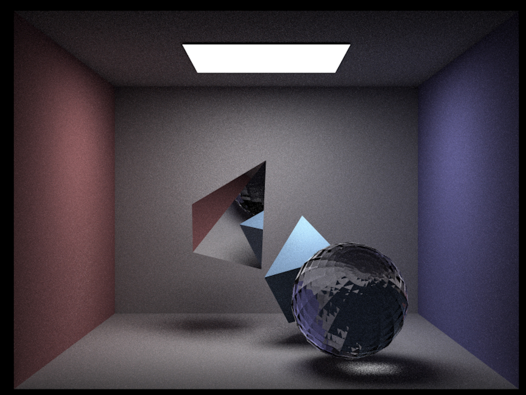
Figure 1: Image rendered by our ISPC path tracer. Note: this image directly contains the path tracer color output, which is in linear space. We did not implement gamma correction or tone mapping, which is why it may look dim at some places.
Performance Comparison with respect to Vector Widths
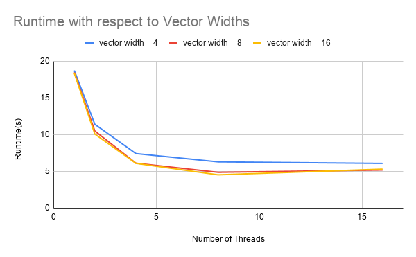
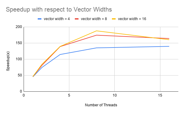
Figure 2: Performance comparison graphs of ISPC implementation with different vector widths
Figure 2 presents the results of speedup comparisons of different vector widths with respect to sequential C++ implementation. We can observe an improvement from vector width = 4 to vector width = 8, though less than 2x difference, but we barely see any improvement from vector width = 8 to vector width = 16, which reveals that we might be suffering from poor vector lane utilization when the vector width is large. More details are explained in the limitations section.
Performance Comparison with respect to Data Size
Figure 3: Performance comparison graphs of ISPC implementation with different data sizes
Figure 3 presents the results of speedup comparisons of different data sizes with respect to sequential C++ implementations. We compared how our program scales with image size of 800x600px, 400x300px and 200x150px. As shown in the graph, our program scales pretty well as data size increases in general. There is a slight drop when the data size becomes large (800x600). We suspect that this can be accounted by the syncing of ISPC tasks. As the data size increased, there are more batches of pixels of rays to be rendered, and after each batch, we will need to sync and wait for previous tasks to finish. With image of larger size, sometimes the load imbalance of different tasks could lead to syncing time increase, which slightly decreased the speedup. Other factors such as machine processing other tasks at the same time could also slightly influence the speedup performance. Since we are still processing a batch of pixels with the batch size being the same as before, this result is likely not influenced by task size or memory issues such as false sharing.
Performance Comparison of BVH on ISPC and C++
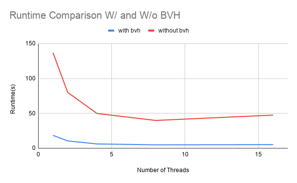
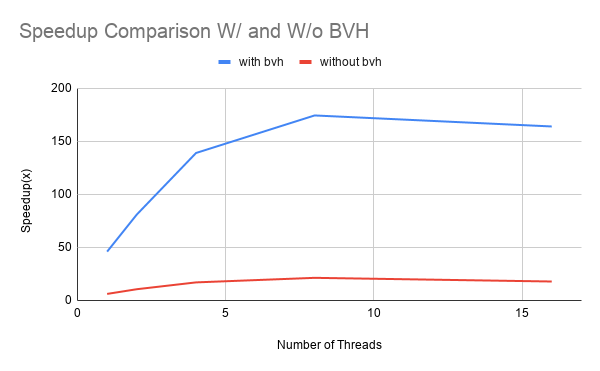
Figure 4: Performance comparison graphs of ISPC implementation with and without BVH optimizations
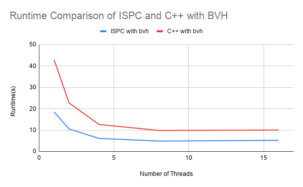
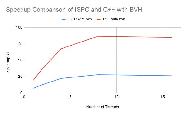
Figure 5: Performance comparison graphs of ISPC and C++ implementations with BVH added
We compared the runtime and speedup of ISPC implementation with and without BVH against C++ sequential implmentation. As is shown in figure 4, we observed that with BVH, the runtime of our ISPC implementation is significantly reduced compared to without BVH, with speedups from 21x to 175x on the scenes we tested. This is expected, as BVH can at-best reduce the number of primitives to test from O(N) to O(log N). We also observed super linear speedup after adding BVH as it reduces the total amount of computation by pruning some branches of the rays as explained in the previous section.
To measure the speedup effects of BVH alone, we compared ISPC implementation with BVH against ISPC optimized single core implementation, and C++ with BVH against C++ sequential implementation, as shown in Figure 5. We did notice that, due to instruction stream branching, the C++ implementation appears to benefit more from BVH alone than ISPC. Since ISPC already optimized based on rays branching and vector utilization, BVH could potentially overshadow some of these efforts, introducing runtime overhead, where C++ originally does have a relatively divergent paths branching with little overhead.
We did not achieve super linear speedup for ISPC implementations without BVH optimizations. Because of runtime overhead, ISPC without BVH still need to conduct auxiliary operations to improve locality and vector lane utilization, such as rays reordering and task mapping. Moreover, memory bandwidth can also become a limitation in terms of data transferring, memory reads and writes. Therefore, these factors prevent our program from achieving linear speedup.
Limitations and Improvements
As demonstrated above, our program achieved speedups that exceeded our expectations. However, there are still some speedup limitations that we noticed from the performance graphs.
Due to difficulty in measuring time directly in ISPC, we did not have direct data measuring the percentage of runtime in different proportion of our implementation. However, we could split our implementation into the following components: generating rays, tracing of single ray, rays reordering and results outputting. We mainly found out that the portion of tracing the single ray can be further improved in terms of optimizing BVH, and rays reordering could also be further improved in terms of data movement. More details are explained below.
First, we can clearly observe that all speedups have relatively small improvement after 8 threads. This is due to the fact that our machine used only has 4 cores, and 8 threads are already enough to hide latency through context switch.
From the graphs shown in Figure 2, we can also demonstrated that as vector width increases, the performance didn’t scale quite well. This shows a potential problem of poor vector lane utilization (we are not able to directly measure the utilization through ISPC). For our experiment, we let all threads evenly split an array of 2048 ray tasks, and with number of threads being 16 for example, we have 64 ray tasks split to each core. With vector size 16, as some rays start to finish, it’s quite possible for the task to not have enough rays to fill one or two vectors, leading to poor vector lane utilization. As a result, the improvement from vector widths is not obvious. However we observed that, inside the trace_ray function, there are many if checks which decides, for exmaple, the form of lighting when tracing a ray. Since SIMD execution would go through the steps for both cases satisfying and not satisfying the if condition, the runtime could be doubled. As a result, we suppose that rearranging the trace_ray function by splitting the if conditions and apply them to rays that are pre-gathered could potentially improve SIMD utilization.
The vector utilization problem mentioned above could be further improved by reordering inconsistent rays in BVH. Toward the end of the project, we ran out of time to further optimize bounding volume hierarchy on the ISPC implementation, which currently introduces a lot of instruction stream branching. We plan to reorder rays similar to how we gather rays after each bounce so that only unfinished rays continue to be traced. Similarly, we can gather rays each time they traverse down the BVH tree for several levels, and group together rays that need to traverse down the same tree branch. This will involve splitting the recursive call to traverse down BVH tree into multiple calls (each all traverse down only one or a few levels), and splitting trace_ray into two phases - before and after BVH traversal (we implemented this far) and inject the actual ray re-ordering code during BVH traversal. In addition, we can also reduce the unit of vector to single ray when the vector utilization drops below a threshold to reduce the number of idle vector lanes.
Moreover, from what we observed in our code, data transfer still remains a problem. For example, as described previously, whenever we gather or sort rays, instead of doing it in place, we need to copy the rays due to parallel scan and sorting. This process significantly drags our performance. Also as demonstrated above, building upon our idea of sorting indices and only copying the data to the temporary array when tracing the rays, we suppose that prefetching can somewhat help with improving the runtime. However, with our current loop structures, the rays are reordered and traced in the next iterations immediately, leaving relatively insufficient time for prefetching to hide the latency. Therefore, we suppose that rearranging the loops by splitting the ray tasks into groups, alternatively sorting and tracing rays would give us enough time to prefetch the indices from the reordered indices array and fetch the rays corresponding to those indices.
For this project, to conduct a thorough experiment analyzing different aspects of the performance on CPU, we did not port our code to CUDA and compare the performance of CPU and GPU. Although, seeing from our results, CPU appears to be also strong enough to provide significant speedups. Due to machine core limitations, with large data size, our machine is not always able to render results in real time. We believe that if we test on GPU, we are likely to see some further improvements with stronger computational capabilities of GPUs, supporting faster real time rendering of scenes.
Conclusion
In this report, we introduced our SIMD path tracer we implemented on ISPC. Through algorithmic and parallel computational optimization, we improved the runtime and achieved a 175x speedup with respect to the sequential C++ implementation running on a 4 core Macbook Pro 2019 13”. Although there are still limitations in terms of the runtime, we have analyzed potential reasons and future directions to further improve the algorithm.